1. Introduction

With the development of society and the growing urban population, large underground structures play an important role in modern urban system (Kim et al, 2000). However, many recorded data show that underground structures would be seriously damaged or even collapsed under strong earthquake. In addition, so far, the risk assessment of tunnels has been based on empirical fragility curves derived from existing damage records in preceding earthquake. Therefore, it is necessary to develop a comprehensive methodology for assessing earthquake risk of tunnel structures (Kim et al., 2008).

It is well known that soil-structure interaction (SSI) analysis is one of the major methods to predict dynamic behavior of structures (Choi et al, 2000). Nonetheless, the main deficiency of this method is that the analytical procedure becomes computationally costly and challenging due to the infinite nature of the ground system. Hence, the ground response acceleration method (GRAMBS), an effective quasi-static method that can deal with the interaction of soil and structure behavior, is employed in this research to replace the SSI approach (Katayama, 1990). It notably improves effectiveness by cutting down the analytical time with still ensuring accuracy. In addition, there is an absence of professional guideline to define damage states of tunnels. In this paper, the data on different damage states is obtained by using pushover analyses (so-called static nonlinear analysis), and the uncertainties of material properties which are joined by the Latin Hypercube sampling (LHS). An extensive set of artificial ground shakes/motions are produced performing various levels of seismic intensity and the fragility or fragility curves are finally established by using the maximum likelihood estimates (MLE).

2. Procedure of Fragility Curve Derivation

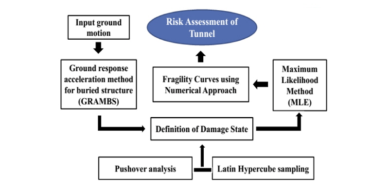
There are number of factors that influence the fragility curve development process such as input ground shake, structural damage data, structural simulation method, analysis method, performance limit states, consideration of uncertainties, etc. Therefore, to establish a frame work for the study, the derivation process used in this study is broken down into sub-tasks as shown in Fig. 1. The proposed methodology is proposed to create a new comprehensive numerical estimation scheme for the fragility evaluation, especially focusing on the integration of GRAMBS and MLE. However, it should be noted that the methodology contains two limitations discussed below. In particular, GRAMBS is not an extensive dynamic analysis method; it is a very effective and efficient quasi-static method that can deal with the soil-structure interaction behavior of underground structures subjected seismic loadings. In addition, the definitions of damage states used in this study might be conservative because they are based on the given numerical model together with consideration of both the performance levels in ATC-40 and the plastic hinges defined in FEMA 356.

2.1 Input ground motion

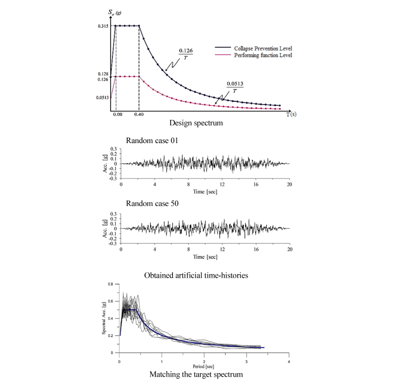
Due to the lack of sufficient and suitable earthquake records in Korea, a set of ground shakes are exploited for the derivation of fragility curves in this study in consideration of the design spectrum mentioned in KBC (KBC 2013). Eleven different seismic levels (IM’s) are considered and 50 time histories of accelerations are artificially generated per each IM by using QuakeGem program (Kim, 2007). Thus, 550 time histories are produced as the input data for the 1-D equivalent linear analysis of free-field ground. Finally, spectral matching is performed and response spectrums are derived for each IM to compare with the design target spectrum. The process is illustrated in Fig. 2.

2.2 Simplified response acceleration method for buried structures

In soil-structure system, the major external force to the structure is provided by the effective dynamic response of the surrounding soil. The dynamic problem of such buried structures certainly becomes the quasi-static interaction problem of the system consisting of a structure and its surrounding soil. When this two-dimensional system is excited by the horizontal input ground acceleration , the equation of motion is provided below (1).

Here [M], [C] and [K] are the mass, damping and stiffness matrix, respectively. X(t) represents the relative displacement vector.

At first, the actual tunnel is neglected and the system is assumed to consist only of the layer soil. The problem therefore turns out to be the free-field response of a uniform soil. The stress of a small portion of the soil from the depth j to j+1 can be expressed as (2).

where Sj represents the stress of the soil from the depth j to j+1, [D] and [B] are the stress matrix, and uj is the relative displacement between the depth j and j+1

When Sj reaches maximum then uj must be maximum and (1) can be rewrite as (3).

Where the right hand side is the dynamic force applied on the whole system at time tm. Because the time is fixed, it becomes the solution of static problem

If the damping of the soil is small, (3) can be approximated as (4).

If the portion of the soil is replaced by the tunnel, then the corresponding parts of the matrices [M], [K], [D] and [B] relating to the calculation of the maximum stress described earlier are replaced by those of the tunnel, and uj becomes equivalent to the ultimate relative displacement between the tunnel’s top and bottom positions. Finally, the ultimate stress state of the tunnel surrounded by the soil is approximately predicted. The analysis procedure for the proposed GRAMBS is illustrated in Fig. 3.

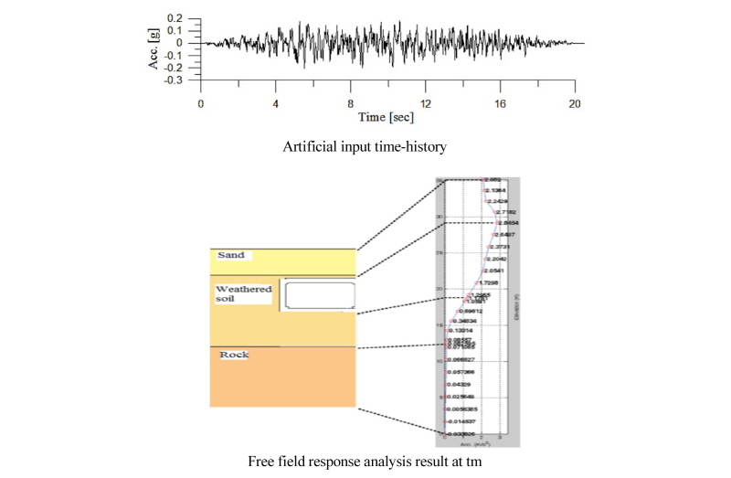
In this study, the tunnel structure is ignored before analyzing the free-field ground response for each sub-layer. One-dimensional equivalent linear method is applied for this purpose based on M-SHAKE software (Kim, 2007). The main target is to estimate the responses of movement and acceleration at each sub-layer against time. Considering the time t_m (at the ultimate relative movement between the top and base slabs of the tunnel, the ground response acceleration at tm is taken all the full length of the ground depth and then converted it into the body forces. The corresponding displacement of the tunnel at time t_m can be obtained by conducting static analysis.

2.3 Damage state definition of two-cell RC box tunnels

Limit states values directly influence the fragility parameters. So, the definition of limit state is a key participant in the development of fragility curves. Although various damage indexes and corresponding parameters have been recommended for the fragility analysis of buildings and bridges, very limited information is available for tunnels. In this study, for damage indexes, the evaluation of damage is based on the deflection response of the structure. The damage states can be divided to three performance levels according to ATC40 (ATC40, 1996): Immediate Occupancy (IO), Life safety (LS), and Collapse Prevention (CP). They can be considered as minor (IO), moderate (LS) and extensive (CP) damage states, respectively. The pushover analysis, a simplified method to survey nonlinear behavior of the structure, is conducted for obtaining the maximum displacement capacity against each damage state.

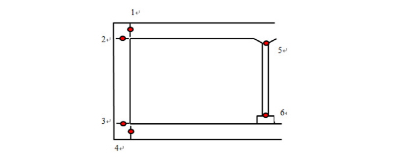
The pushover analyses for the tunnel are carried out using nonlinear finite element analysis program (SAP2000) (www.eqrisk.info). The inelastic behavior of a beam can be modeled by using the concentrated or distributed hinge model. The concentrated hinge model is applied for cases where the yielding will most probably occur at the member ends. The distributed hinge model is applied for cases where the yielding may occur along the member. In this study, the tunnel is considered as a frame structure and the yielding points are assumed to be developed at the end of frames. The hinge positions and typical hinge properties are represented in Fig. 4 and Fig. 5, respectively. AB represents the linear elastic range from unloaded state A to its effective yield B, followed by an inelastic but linear response of ductile stiffness from B to C. C to D shows a sudden reduction in load resistance.

The gradual load increment is applied to generate displacement from initial state to the ultimate. The tunnel is assumed to be placed in one homogeneous ground deposit and two different pseudo-static lateral force models are applied to produce unit displacement at the highest position of the tunnel (Wang, 1993). These models are illustrated in Fig. 6.

(a)Simple model for deep tunnels: The shear force developed at the exterior surface of the roof is the primary cause of the structural racking. Thus, the racking effects of deep rectangular tunnel can be simulated by applying point/concentrated loading at the highest top of the wall.

(b)Distributed load model for shallow tunnels: Due to the decrease in soil cover, the cause of structural racking is shifted to the normal earth pressures developed along the side walls. Therefore, the racking deformation should be imposed by applying an inverted triangular displacement loading along the wall depth.

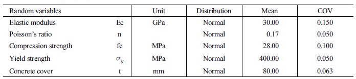
The variability of material strength is often used as a major resource that controls the uncertainty of a reinforced concrete structure. Statistical variation of the material properties can be described by the mean and standard deviation. Thus, random variations and their statistical properties are both used for considering uncertainties, as shown in Table 1 (Matos et al., 2010) . There are several sampling methods can be used to generate random variables. Among the available sampling methods, the Monte Carlo simulation is a powerful tool and is the most widely used. However, there are disadvantages of using this method which is need a very large set of samples to meet the required accuracy. Therefore, in this paper, random variation is produced using the alternative approach, LHS method. This technique provides a stratified-random procedure in lieu of the natural random sampling that used in the Monte Carlo approach.

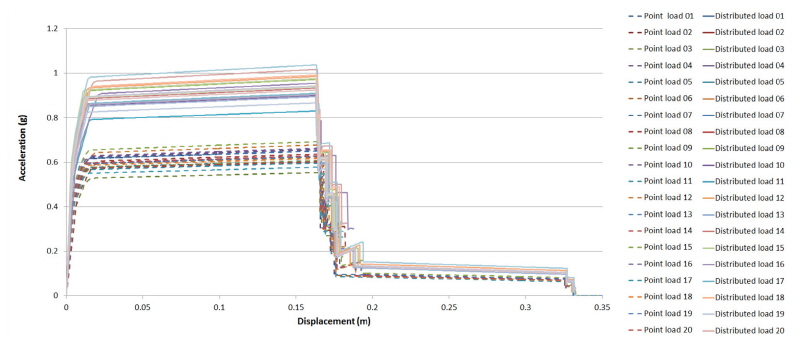
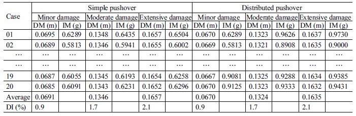
Twenty different pushover capacity curves for each model are described in detail as shown in Fig. 7. The relationship between displacement DM of the tunnel and seismic IM (herein peak ground acceleration) can be clearly acquired from the pushover approach as illustrated in Table 2. The damage index, denoted as DI, is prescribed as the ratio of the horizontal displacement and the height of the tunnel, which can be derived by obtaining the average of drift capacity at each performance level. Four different damage states and their DIs are presented in Table 3.

2.4 Fragility curve development

Response data are obtained in terms of drift capacity. After evaluating the probability of exceedance based on limit states at each earthquake intensity level, the fragility curve can be developed by marking out on a graph of calculated results versus intensity level. The distribution function to represent the fragility curves is considered as follows (Shinozuka et al., 2000)

where P(IM= x) is the probability of failure; , and are the normal cumulative distribution function, the median and standard deviation of ln IM, respectively.

It is common that the failure fragility function is estimated by repeatedly scaling a ground shake until it causes failure of the structure (Vamvatsikos and Cornell, 2004). This process produces a set of IM values affiliated with the onset of failure for each ground shake. Thus, the fragility parameters can be calculated by the Method of Moments (MOM) (Ibarra and Krawinkler, 2005):

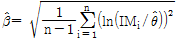
where n stands for the number of ground shakes, IM_i is the IM value affiliated with onset of failure for the i ground shake. 

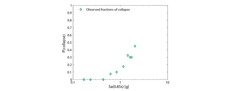
However, the above method is not possible because there is lack of data from past earthquake records. In this approach, selecting different ground shakes at each IM level is chosen in place of using incremental dynamic analysis. Therefore, we do not get an IM value affiliated with the onset of failure for each ground shake, we alternatively have a fraction of ground shake at each IM level that caused failure. Obtained data of this type is illustrated in Fig. 8.

To deal with this problem, two parameters of mentioned distribution function are independently estimated using the MLE method. The likelihood function can be represented by considering each IM level as a Bernoulli experiment (Fitting Fragility Function):

where pj expresses the probability that a ground shake with IM = will cause failure, is the number of failure out of nj ground shakes, m describes the number of IM level.

The final target is to select a function that makes the highest probability of observing failure. Hence, fragility parameters can be gained by maximizing the likelihood function:

The parameters maximizing likelihood function (9) would also maximize the logarithmic likelihood function as shown below

3. Numerical Simulation

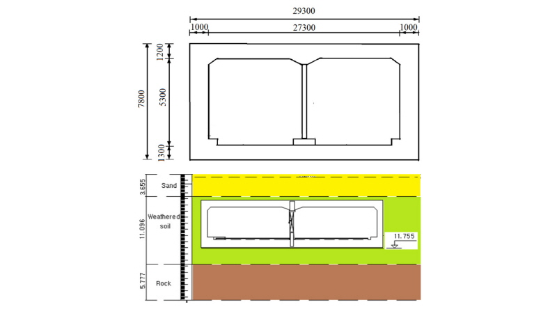
The above concept is cleared up further with the support of a numerical simulation. A real one-story reinforced concrete tunnel with two cells shown in Fig. 9 is simulated. The tunnel height and width are 7.8 m and 29.3 m, respectively. The top and base slabs of the tunnel have their thickness of 1.2 m and 1.3 m, respectively. Deck slab is supported by two side walls with 1.0 m thick and a rectangular column in the middle with the dimension of 0.6 m × 0.7 m. The ground profile has three layers which are sand, weathered soil, and rock base. The soil and concrete properties in this study are summarized in Table 4 and Table 5 in details.

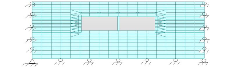
So far, finite element method (FEM) is known as the most powerful technique developed for numerical solution of complex problems in structural mechanics. In this study, a finite element mesh with traditional boundaries is adopted to model structure and soil conditions in Fig. 10. Both the soil and the concrete were modeled as linear elastic materials. The boundary side nodes are restrained vertically (only lateral displacements are possible), while the lower end node is restrained both vertically and laterally.

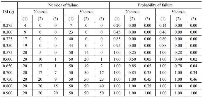
Along all layers, body forces obtained from 1-D equivalent linear analysis by M-SHAKE [4], are applied to the tunnel structures in the static approach. The movements of the tunnel are picked up from static analysis using MIDAS Civil program (Midas Civil On-line Manual 2011). The probabilities of failure for three damage states with two pushover models, as presented in Table 2, are calculated for all eleven earthquake intensity levels in Table 6 where minor, moderate and extensive damage denote (1), (2), and (3), respectively and IM in this example is the peak ground acceleration.

Two statistical parameters as mentioned in Eq. 10 are necessary to construct a fragility curve and the three fragility curves related to damage states are derived for both 20 and 50 cases. The median at each damage state is gained with its corresponding standard deviation summarized in Table 7.

It can be recognized that fragility curves for the three damage states illustrated in Fig. 11 have identical shapes. The number of failures sharply rises with the trivial increase in the earthquake intensity level. The fragility curves gained from this research are found to be similar comparing those proposed by Pitilakis (Pitilakis, 2011). The reason might be due to the difference in the seismic analytical method and damage indexes. Carrying out more cases of pushover analyses can lead more stable results and accuracy of the damage indexes.

In comparison, although the number of sampling increases from 20 cases to 50 cases, there is only a slightly decrease in the obtained value from 0.09 to 0.07 and 0.10 to 0.09 in moderate damage and extensive damage, respectively. It states that the analysis with 20 ground shakes in each IM is a reasonable value for performing structural analysis to derive fragility curves of tunnels.

4. Conclusion and future work

By integrating GRAMBS and MLE, this study has proposed a comprehensive numerical estimation scheme for the fragility evaluation of the two-cell RC box tunnels subjected to earthquake loadings. It is involved with an illustrative example which proves computational effective. Furthermore, according to two-parameters data obtained from the example, the analysis with 20 ground shakes in each IM is considered as a rational value for performing structural analysis. As the same time, a professional guideline for damage states definition is also provided by carrying out pushover analysis and LHS to consider uncertainty of material properties.

The concept can be further extended in years to come by dealing with other uncertainties such as the difference in geometric shapes of the two-cell RC ox tunnels or the variability of soil properties. There are rooms to improve the parameter estimation process for the seismic fragility function. Moreover, although the current research is for tunnel structures, the proposed methodology can be also applied to other underground systems such as pipelines and deep basement structure, etc.