1. Introduction

The behavior of tunnels in hard rocks is mainly controlled by various discontinuities (Ohnishi, 2002). In many tunnels, enormous cost and time are consumed to cope with the falling or sliding of rock blocks, which cannot be predicted because of the complexity of rock discontinuities. It is quite tough to estimate the properties of rock masses before the construction. In the design and construction of tunnels, the observational method has been becoming increasingly important (Hwang, 2003; Hwang and Sato, 2004).

In discontinuous rock masses, rock blocks which have a variety of shapes and sizes are geometrically formed in accordance with their discontinuities. When the rock mass is excavated, the new shape of block come into sight on the excavated surface. The block theory was suggested by Goodman and Shi (1985). Excavations in discontinuous rock masses are frequently affected by key blocks (Ohnishi et al, 1985). The block theory is a useful method to determine the stability of rock blocks that were created by the intersection of discontinuities and the excavated surfaces. However, a key block can be found only after all the discontinuity traces of the block have appeared on the excavation surface. In that moment, the key block is unstable and can be moved out of the surface.

In this study, a new hybrid stochastic-deterministic rock block analysis method for the prediction of the unstable rock blocks before the tunnel excavation is proposed. Using the new hybrid stochastic-deterministic rock block analysis method, the prediction of key block occurrences can be estimated concerning the block surrounded by some discontinuity traces and the cutting face. The new hybrid stochastic-deterministic rock block analysis method in tunnels is applied to a tunnel construction based on actual rock discontinuity information observed in the field.

2. Stochastic Method

The size, location and frequency of key block occurrences are controlled by the number, size, location and orientation of the discontinuities which intersect the excavation. To provide a prediction of expected size and frequency of key block occurrences, it is necessary to consider variabilities of the orientation, size and location of discontinuities.

Spatial location of discontinuity can be described using the coordinates of its center point. Usually, the absolute location is of less interest than the location relative to other discontinuities, particularly those within the same set. Intensity, the number of discontinuities per unit line length, is then used to describe distribution. Spatial location of discontinuity can be determined by a regular deterministic or stochastic process. The most often used model to define the discontinuity spatial location is Poisson model. In the Poisson model, each discontinuity is generated independently; spatial coordinates of its center are generated through a uniform distribution disregarding the locations of formerly generated discontinuities. The number of discontinuities that would be generated is controlled by only one parameter, the intensity parameter that specifies the average number of discontinuity centers within a unit volume of rock mass.

Some models incorporating spatial relationships of discontinuities have been suggested, e.g., Levy-Lee model, nearest-neighbor model, war-zone model, etc. Long and Billaux (1987), and Billaux et al. (1989) have presented a “mother-daughter” process. Mother discontinuities are larger-scale discontinuities, and daughter discontinuities are discontinuities around the mothers. The models that incorporate the relationship among varied scales of discontinuities have a higher-level requirement for in-situ characterization of rock discontinuities.

To determine how many discontinuities would be generated within a specified volume of rock mass, discontinuity intensity is a necessary parameter. In this study, there are three kinds of discontinuity intensities, one-dimensional intensity (i1), two-dimensional intensity (i2), and three-dimensional intensity (i3). And,

i1 = the number of discontinuities encountered by unit length of a borehole that is drilled along the mean direction of discontinuity unit normal.

i2 = the number of discontinuity centers within the unit area of outcrop or excavation.

i3 = the number of discontinuity centers within the unit volume of rock mass.

Among the three intensities, i1 and i2 are in situ measured parameters. Three-dimensional intensity i3 would be inferred from i1 or i2. Parameter i3 is of special importance because the number of simulated discontinuities within modeled region is directly determined by it. Regarding the estimation of i3 for a set of randomly oriented discontinuities, Cacas et al. (1990) used a simple relationship, SI = 2f (S is average discontinuity area; I is three-dimensional intensity; f is discontinuity frequency observed along a core). It is obviously an empirical equation. U.S. National Committee for Rock Mechanics, suggested a simple relationship,

where, NL is discontinuity frequency along sample line; NV is discontinuity frequency within the volume of rock mass; A is mean discontinuity area; is the angle between the discontinuity poles and sample line.

According to this relationship, when assuming that a discontinuity is disc-shaped, one may demonstrate that the relationship between i1 and i3 is,

where, E(I2) is the mean value of the squared discontinuity diameter.

Kulatilake et al. (1993) have employed a little varied relationship,

where, = unit normal vectors of individual discontinuities; = the mean unit normal vector of discontinuity set n.

In a Poisson model, if the volume of rock mass of modeled region is V, the three-dimensional intensity of discontinuity set n is , the number of generated discontinuities within the modeled region would be,

After the generation of simulated discontinuity network with Equation (2) or (3), one may check the discontinuity intensity of the simulated network once again. It is not unusual that the simulated discontinuity network leads to an intensity i1 that differs from the measured one. This may be ascribed to the fact that,

(a) Equation (2) and (3) assume that discontinuities are disc-shaped, but actual discontinuities are not the case. And i1 is an in-situ parameter; (b) In the two equations, only the mean of areas and orientations are respected. Three-dimensional intensity is not only controlled by the mean of area and orientation, but also influenced by the distribution patterns of them.

To overcome this difficulty, in this study a correcting coefficient, Cn, is added to Equation (2). That is, the number of generated discontinuities will be calculated by the following equation,

Coefficient Cn is one of the calibrated parameters. It will be determined through inverse method. In the inverse approach, Cn will be modified in such a way that the simulated discontinuity network will produce the same trace length and one-dimensional intensity as the observed.

Regarding discontinuity population, an outcrop or an excavation may provide more accurate information than a borehole or a scan line. The one-dimensional intensity measured along a scan line is often biased by the scan line direction. It is almost impossible to obtain an acceptable one-dimensional intensity if the scan line is sub-parallel to the discontinuity plane; and it is not easy to prevent a scan line from being parallel to the discontinuity plane when the number of discontinuity sets is reasonably large. When the discontinuities of a rock mass are mapped on some excavation surfaces and some boreholes which are not sub-parallel to the excavation, this study recommends the following equation to estimate the number of discontinuities existing in a given volume of rock mass (V).

where, Cn is a correcting parameter, f1 is the discontinuity frequency along the boreholes.

Naturally, in this study, either Equation (5) or (6) only provides an initial estimation of discontinuity numbers (when there are mapped outcrops or excavations use (6); when there are only boreholes and scan lines use (5)). The exact number of discontinuities in a given volume of rock mass will be determined through an inverse approach.

Discontinuity orientations in three-dimensional space are represented by two parameters, the strike and dip. Discontinuity orientations are not purely random. Discontinuity orientations are usually stochastic and probability distributions are used to describe them. Usually, many of the discontinuities observed in a single outcrop are approximately parallel to three to five planes. These discontinuities, which have approximately the same orientation, constitute a discontinuity set. In most cases, various discontinuity sets are investigated separately. And, in most studies, if not all, discontinuities are clustered into sets with regard to their orientations. Fisher distribution, Bingham distribution, Bivariate Fisher distribution, Bivariate Bingham distribution, Bivariate Normal distribution, and Empiric distribution are the commonly employed distribution forms to represent the distribution of discontinuity poles.

Fisher distribution is most often employed to represent the distribution of discontinuity orientations. In this section, the application of Fisher distribution will be discussed in detail. As shown in Fig. 1, a discontinuity may be represented by its unit normal OP. Suppose that is the angle between the Z-axis and the line of OP in the clockwise direction while is the angle between the X-axis and the line OQ in the anti- clockwise direction where the point Q is the foot of perpendicular P on XOY plane.

After rotating the Z-axis to the direction of the mean pole (, ), the density function of Fisher distribution in the new coordinate system, the random pole (, ) is (Mardia, 1972),

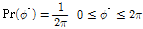
The following property of Fisher distribution makes it very simple to generate Fisher distributed random numbers. And, this may be a reason that leads to Fisher distribution being widely accepted. The property is,

where, 〈〈 is the probability when 〈〈.

The relationship between the new coordinates (, ) and the old coordinates (, ) are,

where, (l, m, n) and (, , ) are the direction cosines corresponding to (, ) and (, ) respectively.

As shown in Fig. 1, they are defined by,

In geology, the data of discontinuity orientations are often given in dip direction and dip angle (, ), not in (, ). As shown in Fig. 1, if the x-axis is oriented to the East and the Y-axis to the North, the relationship between (, ) and (, ) is,

Fisher distribution is specified by only one parameter, which is a concentration parameter: for =0, the polar points are uniformly distributed; for large , the polar points are concentrated on a small portion of the sphere around the pole of the mean direction.

To generate a set of Fisher-distributed discontinuity orientations with specified mean dip direction and dip angle includes the following main steps,

(1)First, compute the mean pole (, ) from the mean dip direction and dip angle with Equation (17).

(2)Generate random-number pairs that follow the specified Fisher distribution (specified by given ), i.e., (, ), i=1,2,···, n (n = the number of discontinuities). The two random-number and are generated inde-pendently. Random variable is uniformly distributed from 0 to 2π.

(3)Rotate the coordinate system back to the old system to calculate (, ) from (, ) through Equation (11) to (16). In the old coordinate system, the X-axis is oriented to the East and the Y-axis is oriented to the North, and the Z-axis is upward.

(4)Finally, transform discontinuity poles (, ) to dip direction and dip angle (, ) with Equation (17).

3. Hybrid Stochastic-Deterministic Rock Block Analysis Method

All discontinuity geometric characteristics may be defined either deterministically or stochastically. A stochastically modeled discontinuity network offers potential for more realistic assessment of stability status in underground excavations than predictions based entirely on deterministic discontinuities. The reliability of probabilistic models, however, depends strongly on an accurate estimation of the models variables, i.e., the discontinuity network properties from the field and laboratory observations.

In this paper, a rock discontinuity system consists of some observed deterministic discontinuities and some stochastic discontinuities. Deterministic discontinuities refer to the discontinuities whose geometric parameters have been determined through certain survey techniques.

3.1 Target polygon for the analysis

It is essential to predict the existence of key blocks which would be formed by the excavation. The geometry of a key block on the tunnel wall is in the form of a finite polygon which is surrounded by some discontinuity traces. Therefore the geometry of that key block which appears partially on the wall, is in the form of a polygon which is surrounded by some discontinuity traces and a face (Fig. 2).

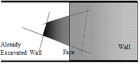
The hybrid stochastic-deterministic key block analysis method is applied to such a polygon. The probability of a removable block occurring by the next excavation can be calculated using rock discontinuity distribution data which are obtained from discontinuity survey on the already-excavated surface.

In general, two discontinuity traces (the upper discontinuity A, the lower discontinuity B) of the target polygon intersect the face. Two discontinuity traces are interconnected directly or connected by some discontinuity traces (linking up discontinuities L) on the already-excavated wall.

The target polygon for the key block analysis is divided into the divergence type and the convergence type on the basis of the directional relationship between the discontinuity A and the discontinuity B on the wall which will be exposed by the next excavation. If the objective polygon is a part of the key block, it is necessary that one of the following events, Ud and Ui, is at least occurred;

(1)Direct connection case (Ud): Discontinuity A and discontinuity B are interconnected directly on wall.

(2)Indirect connection case (Ui): Discontinuity A and discontinuity B are connected by hidden discontinuity H on wall.

3.2 Hybrid stochastic-deterministic simulating procedure

The hybrid stochastic-deterministic simulating procedure process consists of four main steps:

(1)Input observed deterministic discontinuities

(2)Construct random variables generator

(3)Simulate rock discontinuity system with Monte Carlo Method

(4)Improve variables generator with inverse method

When determining the criterion for the good match between simulated and observed discontinuities the following factors are respected:

(1)The mean of trace length on excavation surfaces and/or outcrops

(2)The standard deviation of trace length

(3)1D intensity along boreholes or scanlines

(4)2D intensity on excavation faces.

In the inverse method, the goal function (Press et al., 1989) is designed as below.

where, N = the number of discontinuity sets; = mean length of simulated trace of discontinuity set n; = mean length of measured trace of discontinuity set n; = standard deviation of simulated trace of discontinuity set n; = standard deviation of measured trace of discontinuity set n; = simulated 1D intensity of discontinuity set n; = measured 1D intensity of discontinuity set n; = simulated 2D intensity of discontinuity set n; = measured 2D intensity of discontinuity set n.

4. Application to the Actual Tunnel

4.1 Study area and tunneling method

The actual example site selected in this paper is the tunnel in the New Second Meishin Expressway between Nagoya and Kobe in Japan. The new observational design and construction method for rock block evaluation of tunnels is applied to the tunnel with a large cross-section of about 200 m2. The large tunnel in the New Second Meishin Expressway is now under construction. This tunnel construction is the world's  first large and long tunnel construction which is based on block theory.

The Second Meishin Expressway that will be important to the Japanese economy in the 21st century, is under construction and has been designed to enable cars to travel safely at speeds up to 140 km/h, which will make it by far the fastest expressway in Japan. To accommodate for high speed driving, the curvature of the expressway becomes smaller and tunnel length becomes longer. The cross-section of the tunnel is big. The new road takes three lanes in each direction. The long tunnel in the New Second Meishin Expressway is about 4000 m long.

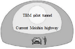
Fig. 3 shows the standard cross-section of the tunnel. The standard cross-section of the tunnel is larger (200 m2) and wider (18 m) compared to ordinary tunnels. The final tunnel shape is a height to width ratio of 0.65. The 5 m diameter TBM pilot tunnel is at the center in the proposed tunnel. After the TBM pilot tunnel is excavated, the main tunnel is enlarged by New Austrian Tunneling Method (NATM).

The TBM Pilot and Enlargement Excavation Method, in which a pilot heading is excavated efficiently in advance utilizing the TBM capability for high speed excavation, is expected to provide various beneficial effects including drainage into the pilot and stability of the face. First, a working tunnel, which was 300 m long, was excavated about 1 km to the west from the east portal because of the topographical condition and the temporary storage yard of muck waste. Next, a pilot tunnel by TBM was excavated to the west. Finally, a pilot tunnel is now under enlargement by NATM.

4.2 Geographical and geology

The district around the tunnel belongs to the Inner Side of Southwest Japan and consists, topographically, of the mountains and the hilly lands distributed on both sides of the mountains. The mountainous region around the tunnel is 300 to 600 m above sea level and a comparatively gentle slope is seen at the summit of the mountains. In addition, steep V-shaped valleys developed along the swamp and river around the tunnel. The Mountains are composed of the Paleozoic formations which are thought to be of Permian age, the granitic rocks which intruded into these formations during the Cretaceous, and a small amount of metamorphic rocks. In the hilly land, Miocene and Plio-Pleistocene strata and Quaternary terrace, fan and talus deposits are distributed. These members rest upon the pre-Neogene rocks unconformably or occur in fault contact with them. The geology of the tunnel mainly consists of Tanakami granite (Collaborative Research Group for the Granites around Lake Biwa, 1982; Kimura et al., 1998; Miyamura et al., 1981) from the Late Cretaceous. The Tanakami granite is a massive coarse-grained biotite granite with equigranular texture. The Tanakami granite is fresh and hard. The maximum unconfined compressive strength is 100 MPa and seismic velocity (P-wave) is more than 4.7 km/s. However, a lot of small-scale faults and fractures are distributed in this area. The longitudinal section is shown in Fig. 4.

4.3 Introduction of block theory

The actual tunnel selected in this paper is one of the large tunnels of the New Second Meishin. Rock blocks around the tunnel have a possibility for rock masses to fall or slide along rock discontinuities not only because the rock mass has a lot of rock discontinuities, but also because the cross-section of the tunnel is large. Therefore, a block theory was introduced based on the behaviors of discontinuous rock mass during the construction of the tunnel as well as after opening it to the public.

4.4 Prediction of unstable rock blocks

The prediction of key blocks using the proposed hybrid stochastic-deterministic key block analysis method in the large tunnel was performed before the tunnel excavation. The key blocks were predicted before all the discontinuity traces of the blocks have not appeared on the cutting face of the tunnel, in other word, in the moment some of the discontinuity traces of the block have appeared. The large tunnel was modeled as shown in Fig. 5. In this section, the predicted key blocks are compared and examined with key blocks occurred actually.

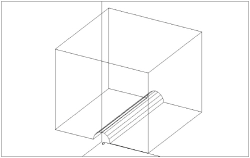
Table 1 shows the distribution of discontinuity data acquired from the investigation of the advancing drift with TBM. Fig. 6 shows key blocks detected by using deterministic key block analysis method. Key blocks predicted using the hybrid stochastic-deterministic key block analysis method are shown in Fig. 7. The key blocks predicted using the hybrid stochastic-deterministic key block analysis method shows a good match with that detected using deterministic key block analysis method. The comparisons and examinations with the analytical results have confirmed the validity and applicability of this hybrid stochastic-deterministic key block analysis method for observational design and construction method in actual tunnels.

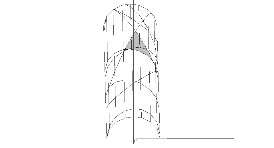
Parameter estimation is a process to find the appropriate parameters that lead to a satisfying match between model-simulated result and observed data. Fig. 8. shows the converging value of the goal function in the inverse method at the actual tunnel. The goal function becomes from 1.9 to 1 by the iteration.

5. Conclusions

In this study, a newly developed hybrid stochastic-deterministic rock block analysis method for the prediction of the key blocks before all the discontinuity traces of the blocks have not appeared on the cutting face of the tunnel is proposed, and then applied to a tunnel construction based on actual rock discontinuity information observed in the field. The comparisons and investigations with the analytical results in the tunnel construction have confirmed the validity and applicability of this new hybrid stochastic-deterministic rock block analysis method in tunnels. The probability of occurring a unstable rock block by the next excavation can be calculated using rock discontinuity distribution data which are obtained from discontinuity survey on the already-excavated surface. In general, stochastic methods are often not effective to analyze local problems which are important for the active support design. In fact, this new hybrid stochastic-deterministic rock block analysis method is also made up on the basis of stochastic theory. However the target of this analytical method is the appropriate local problems.