1. Introduction

In urban tunneling, deformations behavior around tunnel due to excavation may significantly affect nearby structures.

With recent development in computation technology, numerical analysis has been applied to the predicted problem of deformation behavior in urban tunneling on shallow depth and unconsolidated soil. When samples of unconsolidated soil, such as dense sands and stiff clays, are subjected to compression test, it is possible to observe a loss of the overall shear resistance of the specimen with increasing deformation, after a peak load level has been reached (Cividini and Gioda, 1992). Generally, when excavating of a shallow tunnel in unconsolidated soil, it is the particular interest to identify possible deformation mechanism involving strain localization as formation of shear bands developing from tunnel shoulder reaching to the ground surface (Adachi et al., 1985; Gioda and Locatelli, 1999; Hansmire and Cording, 1985; Lee and Ryu, 2010; Sakurai and Akayuli, 1998; You et al., 2000). The various numerical analyses were proposed to explain the shear band development (Adachi et al., 1985;  Kim et al., 2005; Sakurai and Akayuli, 1998; Sterpi, 1999; Sterpi and Sakurai, 1997).

Some researchers have studied the development of shear band using strain softening model (Gioda and Locatelli, 1999; Sakurai and Akayuli, 1998; Schuller and Schwiger, 2002; Sterpi and Sakurai, 1997). Sterpi (1999) conducted strain softening analysis in which strength parameters were lowered immediately after the initiation of plastic yielding. Schuller and Schweiger (2002) demonstrated that the development of plastic shear strains leading to a failure mechanism involves shear banding captured with a Multilaminate model.

Wong and Kaiser (1991) described that deformation mechanisms of the circular tunnel in cohesion-less soil are significantly affected by the variations in key design parameters, such as mechanical properties of soil, horizontal stress ratio, shotcrete thickness, rock bolt effect, excavation modeling, and so on.

This paper investigated the effects of key design parameters affecting deformation behavior by the improved numerical modeling analysis. The numerical parametric study was performed by the proposed non-linear modeling analysis with the various key design parameters, such as the reduction of shear stiffness and strength parameters, horizontal stress ratio, cohesion and shotcrete thickness.

2. Deformation mechanism of shallow tunnel from literature review

One possible explanation of this deformational behavior may be best stated with the help of an illustration given in Fig. 1. Region-A, surrounded by slip plane k-k, is regarded as a potentially unstable zone that may displace downward at the lack of frictional support along vertical k-k planes. The separating region-A from the surrounding is a shear band a formed along k-k line with some thickness, as region A slides downward. The adjacent region-B follows the movement of region-A, leading to the formation of another shear band b. Regions A and B correspond to the primary and secondary zones of the deformational behavior have been pointed out earlier by Murayama and Matsuoka (1969) in the series of trap door experiments. However, it is regarded as a very important fact that a reliable method can be established in order to reveal non-linear deformational mechanism and identify the state of deformation with reference to an ultimate state that is the current interest in the new design practice.

3. Nonlinear numerical modeling

3.1 Anisotropy demage parameter m

Many models have been used to provide some useful results for analysis of geotechnical problems. Sakurai and Akayuli (1998) suggested the anisotropic damage model which combines the anisotropic behavior of rocks with the induced damage that the rock mass undergoes when it is subjected to external forces. From the results of laboratory tests carried out on sand specimens under unsaturated conditions and other geomaterials, Sakurai and Akayuli (1998) found out that the secant Young's modulus, E, is constant throughout the specimen and does not change with load while shear modulus, G, decreases as the applied load increases. The damage occurs along 'slip' planes that are defined as planes of potential failure along which failure can occur when the external stress reaches a certain level.

Fig. 2 shows the relation between m and shear strain in soft rock and sandy ground (Sakurai and Akayuli, 1998). As the loading on the material increases, then m (=G/E) decreases due to the induced anisotropic damage of the material that increases as a result of the external loading.

3.2 Reduction of strength parameters

Sterpi (1999) conducted the strain softening analysis in which strength parameters were lowered immedi-ately after the initiation of plastic yielding. That is strength parameters were reduced from the moment of initiation of yielding to residual values, as indicated in Fig. 3.

This implies that the admissible space for stress is gradually shrunk as strain-softening process takes place. In this diagram, ci is the initial value of cohesion, cr is the residual value, φi is the initial value of friction angle, φr is the residual value, and △ϒ is the increment of maximum strain during which strength drops from peak to residual value.

3.3 Used nonlinear modeling

The used model incorporates the anisotropic damage parameter, m (=G/E), as well as strain softening effects of strength parameters, cohesion c and friction angle φ.

Following is a brief summary of fundamental cons-titu-tive relation between stress, σ, and strain, ε.

The x' direction coincide with the slip plane while the y' is the plane of symmetry and is perpendicular to the plane of isotropy. A fundamental constitutive relation between stress, σ', and strain, ε', is defined by a equation (1) and (2) defined for a local coordinate system shown in Fig. 4 (Akutagawa et al., 2006).

                              (1)

(2)

The constitutive relationship is defined for conjugate slip plane direction (45º ± φ/2) and transformed back to the global coordinate system. Eq. (2) can be trans-formed to global coordinates as follows;

                     (3)

where, [T] is a transformation matrix. When damage has not occurred, the relation holds, and matrix [D'] is identical to [D]. The stress strain relationship for the global coordinate system is given in the following form;

                                (4)

      (5)

An anisotropic parameter m is defined to be the ratio of G to E and expressed as(Sakurai and Akayuli, 1998);

                     (6)

where Poisson ratio, , is assumed to be constant. The damage parameter, d, can be expressed as a function of the shear strain along the slip plan as (Sakurai and Akayuli, 1998);

       (7)

where me is the initial value of m, mr is the residual value, α is a constant, is shear strain, is the shear strain at the onset of yielding. However, m is lowered immediately after the initiation of plastic yielding.

The proposed nonlinear analysis is reduction of shear stiffness and strength parameter after yielding (namely, strain softening). Those are, an anisotropic parameter, m (=G/E), and strength parameters, c and φ, which are reduced from the moment of initiation of yielding to residual values, as indicated in Fig. 5 (Akutagawa et al., 2006).

This implies that the admissible space for stress is gradually shrunk as strain-softening process takes place.

Any excess stress, which is computed on the trans-formed coordinate system based on slip plane direction, outside an updated failure envelope is converted into unbalanced forces that are compensated for in an iterative algorithm. Fig. 6 shows the used numerical analysis flow, where, [B] is a strain-displacement matrix, m is an anisotropic parameter, G/E, [D] is stress-strain matrix, and [K] is stiffness matrix, {f} is force vectors, {△u} is calculated displacement vectors, {△ε} is strain and {△σ} is stress.

4. Effect of soil material parameters and initial horizontal stress in deformation behavior around tunnel

4.1 Numerical modeling

A cross section of a shallow tunnel has been modeled. The tunnel overburden was chosen to be roughly the same as the tunnel diameter (z/d=1). Due to symmetry in the geometry, only the right half of the tunnel has been analyzed. The analysis domain has an extent of 35m × 37m with horizontal fixities at both sides of the mesh. The bottom nodes of the mesh are vertically fixed. Boundary conditions of the finite element mesh are presented in Fig. 7. In Fig. 7, the medium mesh consisting of 631 finite elements is presented. Tunnel diameter is 10m. Excavation of the full tunnel face is modeled by gradually released load associated with excavation. In each load step, the system is loaded 2% of the total excavation forces.

Fig. 8 shows the observed points in numerical analysis. In Fig. 8, surface settlement is observed at 16 points with 2m intervals. Subsurface settlement above tunnel center is measured also with 2 meter interval, and the horizontal displacement is measured at 6m away from tunnel center line. Tunnel behavior is observed by the crown measurement, convergence and foot settlement, in Fig. 8 (b). Table 1 and 2 show the basic material properties and parameters pattern for nonlinear behavior effect, as softening parameter. The basic material properties and strength parameters values obtained by lab. test, such as triaxial test so on, in dense sandy.

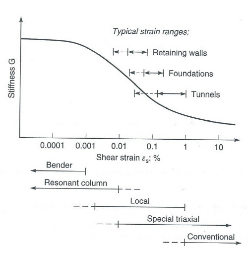
Softening parameters consist of two values is the ration of residual strength to initial strength and is the increment of maximum shear strain during drops from peak to residual value. The boundary of is selected from the reference of Fig. 9(Potts, 2002), as 0.01, 0.02 and 0.04. Table 3 show the properties of the studied parameters values.

4.2 Numerical results

4.2.1 Mesh dependence

To evaluate the possible mesh dependencies, three different meshes having, 631, 1440 and 1758 elements, respectively, were tested. The material parameters are given in Table 1 and 2.

In the first step of the finite element analysis, the initial stress state in the ground prior to tunnel excavation, horizontal stress ration has been calcul-ated by 0.4. Nonlinear softening behavior is defined by the ratio of residual strength to initial strength =40% and the increment of maximum shear strain during drops from peak to residual value =0.01.

Fig. 10 shows the used FEM meshes. The tunnel behaviors and surface subsidence for all three meshes are presented in the diagram in Fig. 11. In the diagram, Frel. represented the released forces and Fexc. means the total excavation forces. Settlements are plotted against the percentage of the excavation forces that has been applied.

Fig.12 shows the maximum shear strain distri-butions for the meshes with 631 and 1440 elements. In Fig. 11and 12, it can be found that the mesh dependency of the deformation behavior and shear band formation are significant as far as the studied examples are concerned.

4.2.2 Influence of softening parameter

For investigation of the effect of softening parameter, analyses with 9 different patterns were carried out as shown in Table 2. The initial stress state prior to tunnel excavation is assumed by K0 = 0.4. Fig. 13 presents the calculated crown settlement, convergence and its relation with the 9 different softening patterns.

Fig.13 (a) crown and (b) convergence shows relatively similar behavior until Frel./Fexc.=40%. After this exca-vation step, crown settlement and convergence start to show different behaviors with the effect of softening parameters.

Fig.14 (a) and (b) showed the calculated subsidence profile due to excavation for Frel./Fexc.=70%, 74%, 78%, 82%, 86% and 90%. Crown settlement and convergence are more developed when softening para-meters decreases, as =40% and =0.01.

Fig. 15 shows the calculated subsurface settlement at 6m away form tunnel centerline due to excavation. The subsidence for =40% and =0.01 is greater than that of =80% and =0.04. Fig. 16 shows the calculated horizontal displacement at 6m away form tunnel center (T.C.) due to excavation.

Fig. 17 represents the maximum shear strain distri-butions for Frel./Fexc.=78%, 82%, 86% and 90%. The maximum shear strain distribution for =40% and =0.01 is growing faster than that for =80% and =0.01. This figure suggests that the develop-ment of shear bands can occur suddenly between Frel./Fexc.=82% and 86%.

Fig.18 represents the maximum shear strain distri-bution at Frel./Fexc.=86% in which a clear relationship between the development of the shear band and softening parameters is recognized.

4.2.3 Influence of horizontal stress ratio, K0

Numerical analysis is carried out with varying K0 value and softening parameters. The horizontal stress ratio prior to tunnel excavation depends on the soil material but it is also a result of the loading history leading to different stress paths at various locations.

The horizontal stress ratio is expressed by the ratio of effective horizontal stress to effective vertical stress.

Numerical analyses have been performed using the material parameters presented in Table 1, 2 and 3. K0 values of 0.4, 0.6, 0.80 and 1.0, respectively, have been used. Fig.19 show horizontal displacements at 6m away from Tunnel center with Frel./Fexc.=86%, as compared with K0 values and softening parameters. In Fig. 19, the horizontal displacement towards tunnel becomes greater when K0 values increase.

The development of maximum shear strain from the various K0 values and softening parameters are depicted in Fig. 20. A low horizontal stress ratio of K0=0.4 results in a relatively large development of maximum shear strains. In this Figure, the strains are concent-rated in a narrow zone rising from tunnel sidewall almost vertically towards the ground surface.

For the higher K0 value, the development of signi-ficant maximum shear strain distribution is restricted to a smaller zone close to the tunnel sidewall.

4.2.4 Influence of initial cohesion value

In the deformation behavior of shallow NATM tunnel with sandy soil, cohesion parameter is one of the important material parameters, which is studied in this section. The initial cohesion values are set to 20 and 40 kPa, and the fundamental parameters included in Table 1, 2 and 3 were used.

Fig. 21 shows the subsidence profile. It is seen from three figures that the behavior is largely different when the initial cohesion drops from 40 to 20 kpa.

5. Effect of shotcrete thickness in deformation behavior around tunnel

The following analysis demonstrates the effect of shotcrete thickness. In the first step, 40% of the normal forces associated with excavation of the top heading have been applied. In the second step, the shotcrete has been put in place and, at the same time, the remaining 60% of the excavation forces have been released.

The fundamental parameters included in Table 1, 2 and 3 were used. Shotcrete was simulated in a simpli-fied way by using a linear elastic model with plane elements and distinguishing only thickness. Fig. 22 shows crown settlement with the variation of shotcrete thickness when =40% and =0.01.

The development of a maximum shear strain for various shotcrete thicknesses and softening parameters are depicted in Fig. 23 for Frel./Fexc.=88%.

The stability is not guaranteed for 0 cm thickness. However, the development of shear zone is confined to narrow bands by shotcrete system of 15 cm, 20 cm and 25 cm.

6. Conclusion

This paper was carried out the deformation behavior of tunnel and ground by numerical parametric analysis using nonlinear model incorporating the reduction of shear stiffness and strength parameters. Numerical para-metric studies are carried out by considering the key design factors affecting ground behavior around tunnel, such as the reduction of shear stiffness and strength parameters, horizontal stress ratio and shotcrete thick-ness. Applied numerical tunnel modeling is only slightly influenced by the mesh fineness. Crown settlement, subsidence and the maximum shear strain distribution are more developed when the ration of residual strength to initial strength and the increment of maximum shear strain decreases. The ground behavior are affected slightly less when the ration of residual strength to initial strength, =80% and the increment of maximum shear strain, =0.04 than =40% and =0.01. A low horizontal stress ratio, K0=0.4, developed a relatively large maximum shear strain than K0=1.0. Regarding the initial cohesion values 20 kPa and 40 kPa, it is seen that the deformation behavior differs greatly when the initial cohesion drops from 40 kPa to 20 Kpa. This analysis demon-strates the effect of shotcrete thickness. While the tunnel stability is not guaranteed for 0cm thickness, the development of the shear zones I sconfined to narrow bands by shotcrete systems of 15, 20 and 25 cm.