1. Introduction

In practice, we meet a number of problems associated with rock joints and discontinuities. In tunnel engineering, stability of supporting columns which contain rock joints or faults is a main concern. And in geotechnical engineering, they have pro-blems such as slope stability, foundation and under-ground openings, which are related to the behavior of rock joints and faults involved. There-fore, joints, faults, and discon-tinuities play a vital role in rock and tunnel engineering practices.

The behavior of the discontinuous joints is different from that of the continuous solid materials. The shear strength of a solid comes from the strong internal cohesion, while the shear strength of a joint is mainly derived from contact friction which involves many types of mechanisms, such as inter-locking, ploughing, and damaging of the asperities. Therefore, the modeling of the joints involves significant comple-xity and is very impo-rtant. Rational constitutive models can only be obtained through careful study of their special features in addition to those of continuous solids, and also through con-sideration of the basic mechanics and labora-tory testing and verification.

This research aims to investigate the strength and deformation behavior of the joints or discontinuities under various loading conditions. The objectives of the investigation can be summarized as follows:

1) To modify the disturbed state concept theory for its application to the rock joint modeling.

2) To develop the model capable of describing and predicting the hardening and softening behavior of the rock joints under various stress path conditions.

3) To utilize the proposed model and verify it with respect to experimental data on rock joints.

4) To analyze the size effect of the joints in mode-lling.   

Several models have been developed for defining the behavior of joint. There are two types of joint models: failure model and elasto-plastic model.

1.1 Failure models

Failure models describe the shear stress in relation to the normal stress and other parameters. This relation is generally nonlinear as long as the range of the normal stress is wide enough. Usually, the shear stress reaches a peak value and then decr-eases to a residual value. This phenomenon is termed softening as found in most rocks (Goodman, 1974; Hoek and Bray, 1974). In failure models, emphasis is focused mainly on the modeling of peak and residual shear stresses.

Barton and Chouby(1977) proposed a failure model for peak shear strength of rock joints after sum-marizing extensive tests upon specially prepared artificial rock joints. The peak shear strength was expressed as

 (1)

where JRC and JCS are the Joint Roughness Coefficient and Joint Compression Strength res-pectively, and is the residual friction angle. Schneider(1975) modified Patton’s bilinear model by combining the angle of asperities of natural rock joints.

Most failure models described the above attempt to relate the shear strength of a rough joint with the slope angle or the shear strength with the strength of the asperities. However, failure models do not give the description of the stress-strain relationship which is necessary for calcu-lations involved with displacements other than the strength of the joints. The elastic and elasto-plastic models are capable of providing the stress-strain relationship as discussed below.

1.2 Elastic and elasto-plastic models

Goodman, Taylor, and Brekke (1971) proposed a nonlinear model for rock joints. This model has the off-diagonal terms of the stiffness matrix which are considered as the coupling terms between the shear and normal behavior. Ghaboussi and Wilson (1973) proposed the possible application of the plasticity theory in joint modeling by assuming the association flow rule. The yield functions used here are the Mohr-Coulomb failure law for non-dilatant joint, and the Cap (DiMaggio and Sandler, 1971) model of yield functions for dilatant joint. Zienkiwicz et al. (1977) proposed an elastic-viscoplastic model for joint. The yield function F used is the Mohr-Coulomb failure law. Both associative and non-associative poten-tial function Q has a similar type as the yield function. Plesha (1987) proposed a non-associative plasticity joint model. The main feature of this model is to use a parameter called the asperity angle to characterize the strength and deformation behavior of the joint. At the same time, Desai and Fishman (1987) developed a non-associative plasticity model by specializing a general 3-D Hierarchical Single Surface model (HiSS Model) (Desai et al., 1984, 1986). The yield function F and the displacement potential function Q are expressed as

 (2)

 (3)

where n and are material constants, is the hardening function, and is the non-associative hardening function. This model can be used for both quasi-static and cyclic loading conditions. However, softening can not be captured.

In this paper, a modified version of Disturbed State Concept (DSC) model (Desai, 1992; Desai, 1995; Park, 1997) is proposed to model both hardening and softening behavior with a frame-work that can include a number of important characteristics of joints

2. Disturbed sate concept modeling for joint of rock

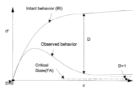
The disturbed state concept (DSC) extends cont-inuum theory representations of material behavior to include observed nonhomogeneous and discont-inuous behavior such as microcracking, damage, and softening. It is based on the DSC that allows incorporation of microstructural changes due to the applied forces, that cause transitions in the material from relative intact (RI) state, through a process of natural self adjustment, to the fully adjusted or critical (FA) state. The process of transition from the RI to FA state involves changes in the microst-ructural properties of the joint material, affected by factors such as roughness, asperities, particle size and shape, and interparticle characteristics. The observed material behavior is thus defined as a combination of the two material reference states, RI state and FA state, which are related through the disturbance function, D (Fig. 1). The concept of the disturbed state of a joint can be expressed by the two reference states (RI and FA) and D.

The disturbed state for a joint is the inter-mediate state from the original state until the critical state is researched. During the disturbed state, the damageable material and non-damageable material co-exist. From the DSC theory for a joint material (Desai, 1995), the damageable material repres-ents those asperities that are broken or lose contact during shearing, and those contacts that are separated by the debris. The non-damageable material repres-ents those asperities that are not breakable for the given normal stress, and would include plateaus formed and compacted gouge material formed during shearing. Consequently, strain softening may result if the joint becomes smoother.

To best describe the various references states for jointed rock, a simple example is presented herein. Consider a bucket filled with ice. When heated, the ice will thaw into water. The ice represents the material in its original state or RI state, while the water represents the material in FA state, and heating is the factor that causes the disturbance, D. During the period starting from ice (RI state) and ending with water (FA state), there are many inter-mediate states where the container includes both ice and water. These intermediate states are said to be in the disturbed state. During the disturbed state, the ice changes gradually to water and there exists a mixture of ice and water.

2.1 Idealization of a joint

A joint is the region of two opposing surfaces of two contacting solids. The physical properties of a joint are determined by these two surfaces and their contact conditions. To mathematically model a joint or interface, the joint is usually considered as a planar surface with two joint walls and a contact space (Fig. 2). Here, the contact space is the contact zone of the opposing asperities and it can be assigned as averaged thickness t. A coordinate system can be established where the planar surface is considered; the tangential direction with shear stresses , and relative shear displacements , and the direction orthogonal to the planar surface is the normal direction with normal stresses , and relative normal displacement . If T and N are the tangential and normal forces applied (Fig. 2), and A0 is the nominal joint area, then the normal and shear stresses are:

 (4)

 (5)

The relative shear displacement , in contact zone is composed of elastic shear deformation of the contact asperities , plastic shear deformation of the contact asperities , and slip displacement between the contact asperities of the joint,

 (6)

In an analogous manner, the relative normal displacement, , can be defined as

 (7)

If small strains are assumed, the joint thickness, t, can be used to convert relative displacements into equivalent strains. As t comes to zero, the in-plane strain converges to zero and can be negligible. In view of this, the in-plane stress, , will also be small and can be negligible, particularly when the Poisson’s ratio, , is small. In terms of two- dimensional idealization, the strain-displacement relations are

 (8)

and the related stress components are

 (9)

2.2 Description of the RI state

The relative intact state is described using the modified HiSS model (Desai and Wathugala, 1987). The model is based on the associative plasticity and isotropic hardening (potential function Q = yield function F) rule. In this model, the yield function, F, is given as:

 (10)

where is the shear stress, is the normal stress, and n and are material parameters. is the hardening function and it is expressed as

 (11)

where a and b are material parameters and trajectory of plastic shear strain, , is given as:

 (12)

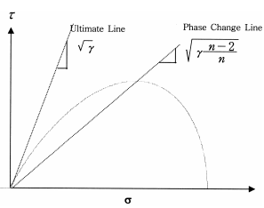
The yield surface F is a continuous set of convex surface which expands toward an ultimate yield surface during plastic shear deformation. The ultimate surface, , which represents the asymptotic failure stress, is found by setting equal to zero:

 (13)

This plots a straight line with slope as shown in Fig. 3. The locus of points expanding yield surface (where the tangent to the yield surface is

parallel to the axis) is a line called the

“Phase Change Line”. By taking F=0 and , Eq. (12) reduced to

 (14)

The phase change line also plots as a straight line

with slope in vs. space (Fig. 3) and

in stress space (Fig. 4).

2.3 Description of the FA state

The critical state is a steady state where the shear stresses and normal displacement are stabilized. The joint model at the critical state consists of two parts: the modeling of the critical shear stress and the modeling of the critical dilation. The failure model proposed by Archard (1958) is a simple one yet it gives a very good description of the shear stress at the critical state. Archard's non-linear power law model can be expressed as follows:

 (15)

where and m are material parameters and the superscript c refers to the critical condition. And the final dilation at the critical state, , is found to have a relation with the normal stress (Schneider, 1975), as

 (16)

where is the maximum dilation when is equal to zero and k is a material parameter.

2.4 Description of DSC function

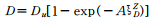
The proposed function for D (scalar) employed in this research was used by Armaleh and Desai (1990):

 (17)

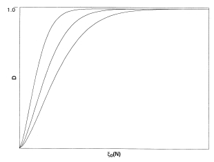
where Du is the ultimate disturbance. Initially with no disturbance the material is assumed to be entirely in the RI state, so D is zero. With full disturbance the material is assumed to be fully in FA state, and at an ultimate state, Du. Theoretically, the disturbance, D, varies between 0 and 1, but many materials fail in an engi-neering sense before D reaches unity. A and Z are material parameters. This disturbance function will be used twice to define a shear stress relationship using disturbance, , and an effec-tive normal stress relationship using disturbance, . Each curve in Fig. 5 is a repre-sentation of Eq. (20).

3. Incremental formulation for back prediction program

3.1 Derivation of the intact incremental stress-strain relation

Derivation of the intact incremental stress-strain relations follows the traditional elasto-plasticity formulation procedure (Desai and Wathugala, 1987). Let the following vectors be defined

 (18)

 (19)

From the elastic stress-strain relationship and the flow rule for plasticity, an incremental form of the intact stress vector can be found as

 (20)

where is the elastic constitutive matrix and is given by,

 (21)

where kn and ks are the normal and shear stiffness of the interface material. And employing the  con-sistency condition of the yield function (dF=0), can be found as

 (22)

and substituted into Eq. (20) to yield the cons-titutive relationship desired,

 (23)

where the elasto-plastic matrix takes the form

　 (24)

where L is defined as

 (25)

for the hardening function defined in Eq. (25) where are McAuley's brackets.

 (26)

3.2 Derivation of the DSC incremental stress equation

Assuming the thickness of joint is the same for all three material phases, equilibrium of forces in the disturbed material, and the definition of distur-bance in Eq. (17), the following relationship between phase stresses can be derived

 (27)

where the normal disturbance function, , can be used to model the relative normal displacements and , is the disturbance function for relative shear displacements.

Differentiating Eq. (27),

　 (28)

If there is no change in stresses at FA state, and are zero. Substituting Eqs. (15) and (23) into Eq. (28) gives the DSC incremental stress- strain equations,

　 (29)

and 

 (30)

where the term contributes negative values during softening and [CDSC] is DSC con-stitutive matrix.

4. Model parameters

The proposed joint model involves a number of material constants which can be determined from a series of shear tests on joints or interfaces. The material constants can be divided into three cate-gories: parameters for RI material, the constants for FA material, and the disturbance function parameters. The material constants are all listed in Table 1. There are eleven parameters needed for the DSC joint model.

5. Verification of DSC model for rock joints

The disturbed state joint model derived and modified in previous section is verified with respect to comprehensive laboratory tests per-formed by Schneider (1974). For verification, the model back predictions are obtained by numerical integration formulation based on Equation(30).

Schneider (1974) performed a series of well designed shear tests. The samples of the joints are replicas made of plaster casts from a same natural rock joints. In doing so, many similar joints samples were produced and the influence of the normal stresses on the joint behavior was studied. For this research, the granite joint is utilized and investigated. The granite joint is relatively rough and has a high degree of indentation both on the microscopic as well as on the macroscopic scale.

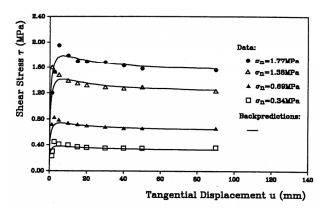
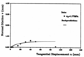
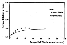
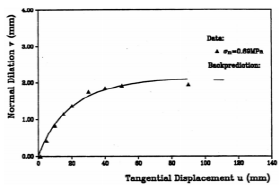
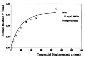
For the granite joint, four tests were performed under different constant normal stresses. The normal stresses are 1.77MPa, 1.38MPa, 0.69MPa, and 0.34MPa, respectively. The back predictions of the four tests are shown from Fig.6 to Fig.10 and model parameters used in the back predictions are listed in Table 2. Fig. 6 shows the back prediction of the shear responses for the four tests under the four different normal stresses. the normal stress σn is kept constant during each test and severe softening occurs for all four tests. Fig. 7 to Fig. 10 show the back predictions of the dilative responses.

predicted softening behavior of the granite joint. The back predictions are very satisfactory for the two shear tests with low value of normal stresses (0.69MPa and 0.34MPa). Reasonably good predictions are shown for the two shear tests with higher normal stresses (1.77MPa and 1.38 MPa), but the high peaks of the shear stresses are not predicted by the back predictions. This is because the material parameters are found through an average process and the number of data points for the high peaks are too few to input a significant influence.

The difference of the normal stresses used in the tests are large enough to cause a significant change in the dilative behavior for different normal stresses from Fig. 7 to Fig. 10. The back predictions for the dilative behavior are very good except for the test with normal stress σn=1.77MPa, where large discrepancy can be observed in Fig. 7. This large discrepancy is due to the non-regularity of the data obtained from the test, possibly due to a catas-trophic damage occurred to the asperities under such a high normal stress and consequently, the dilation reduces to a very small value at large stage of the shear process.

6. Conclusions

The disturbed state modeling provides a powerful way of describing the behavior of joints of tunnel. It is based on the assumption that the behavior of a joint, or the behavior at the disturbed state can be expressed by the joint behavior at its reference states.

The reference states include the original (RI) state and critical (FA) state. Basic models can be used to describe the simple behavior at the reference state and the complex behavior at the disturbed state can be described by using the disturbed state joint model.

From this study, the behavior of intact joint is modeled by using a general plasticity model with minor modifications. The FA state is modeled according to the observations from the shear tests of joints. The DSC joint model based on two reference states thus developed is capable of describing the hardening and softening behavior of a joint under various stress paths.

The model can be easily implemented in numerical integrated formulation procedures and requires a realistic number of parameters for general use. Finally, this model is capable of capturing essential rock joint behavior including strain softening using back prediction scheme.