1. Introduction

The properties of rock masses are very important factors in the design and construction of tunnels. Rock masses in nature contain a great variety of discontinuities such as faults, joints, fractures, bedding planes, seams, cracks, schistosities, fissures and cleavages. The behavior of civil structures in hard rocks, therefore, is mainly controlled by numerous discontinuities (Ohnishi, 2002; Hwang, 2003; Hwang et al., 2004). The tunnel support design has been mostly empirical. The typical support design pattern is based on the rock/soil types, or based on the rock mass classification. However, both stress and rock structure induced failures should be considered in the design of rock support for tunnel design.

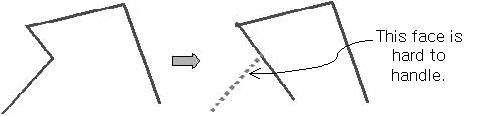
As for the assessment of the rock structure induced failures, the so-called block theory was suggested by Goodman and Shi (1985). Excavations in discontinuous rock masses are frequently affected by key blocks, which are critical blocks of rock bounded by discontinuities and excavation surfaces. Block theory is a geometrically based on set of techniques that determine where dangerous blocks may exist in a rock mass intersecting by variously oriented discontinuities in three dimensions. Block theory is a quite useful method to determine the stability of rock blocks that were created by the intersection of discontinuities and the excavated surfaces. However, the block theory is based on some assumptions which limit its usefulness. In block theory, joint surfaces are assumed to extend entirely through the volume of interest; that is, no discontinuities will terminate within the region of a key block (Ohnishi et al., 1985). The block theory is based on the assumption of infinite persistent discontinuities, and does not consider the effects of finite discontinuity persistence, therefore cannot deal with a complex concave shaped block (Fig. 1). The rock block should be divided into convex sub-blocks. In practice, it is necessary to consider the persistence of finite discontinuities to attempt applying the block theory to successive excavations.

In this study, a new key block analysis method for observational design and construction method in tunnels is proposed, and then applied to the actual large tunnel. Three-dimensional rock block identification with consideration of the persistence of discontinuities is performed by using discontinuity disk model. The removability and stability analyses of rock blocks formed by the rock block identification method are performed. The new analysis method for observational design and construction method in tunnels can handle concave and convex shaped blocks.

2. 3D Discontinuous Rock Mass Modeling

2.1 Discontinuity disk model

To build a 3D model considering finite discontinuity persistence, the problem concerned with geometric shape and spatial extent of discontinuities must be addressed. Through the analysis of trace data and examination of discontinuity surfaces, several studies (Warburton, 1980; Long and Billaux, 1987; Pollard and Aydin, 1988; Priest, 1993; Ohnishi et al., 1994) have demonstrated that discontinuities are likely to be roughly elliptical or circular.

The fundamental basis of the discontinuity disk model is the assumption of circular discontinuity shapes (Ohnishi et al., 1994; Mardia, 1972; Pahl, 1981; Dershowitz, 1984; Kulatilake et al., 1993; Zhang and Einstein, 2000) as shown in Fig. 2.

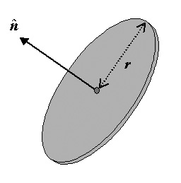
The size of circular discontinuities is defined completely by a single parameter, the discontinuity radius. Discontinuity radius may be defined deterministically, as a constant for all discontinuities, or stochastically by a distribution of radii. The best and most widely adopted sampling strategy for determining discontinuity size is based on the measurement of the lengths of the traces produced where the discontinuities intersect a planar face (Priest, 1993). The probability distribution of discontinuity diameters may be inferred from the distribution of the trace length, which can be measured through excavation surfaces or natural outcrops. However, the direct estimation of trace lengths is often influenced by varied biases, and the distribution inferred from trace length involves integration that can only be evaluated numerically, and this also becomes a barrier when building a statistical model with Monte Carlo simulation. To overcome these problems, the stochastic discontinuity system modeling process of this developed program first assumes that discontinuity diameter and trace length have the same distribution function (e.g., lognormal or exponential distribution), then determines the mean and standard deviation of discontinuity diameters through model calibration. Discontinuity location may also be defined by a deterministic pattern or a stochastic process. The most frequently used model to define the spatial location of stochastic discontinuities is the Poisson model. In the discontinuity system modeling process of this developed program, the spatial location of stochastic discontinuities was assumed to follow the Poisson model. As a result of the discontinuity location, shape and size process of the discontinuity disk model, discontinuities terminate in rock and intersect each other.

2.2 Analysis region modeling

The model region of this study is a closed domain with a certain number of faces. Model region may be of any shape closed by polygons. The excavation faces may be convex or concave polygonal faces with or without interior holes. All excavation faces should form a closed domain of target rock mass for the analysis; if they do not form a closed domain, some fabricated faces, such as boundary faces, should be added. A curve face should be approximated by a number of polygonal faces. Fig. 3 shows an example of the analysis region modeling for an underground cavern.

3. Identification of 2D Loop

In a discontinuity system, not all discontinuities (which may be deterministic or generated by stochastic simulation) are connected; some discontinuities do not intersect with other discontinuities, and some discontinuities intersect with very few discontinuities (Yu, 2000). Before the rock block identification stage, unconnected discontinuities should be identified and eliminated. In order to reduce computational requirement, some discontinuities may be considered unconnected and eliminated because of their small sizes.

A discontinuity is referred to as connected only when it plays a part in block formation (i.e., it forms a surface of some block). A connected discontinuity must feature the two following characteristics: (1) it is connected to at least 3 discontinuities including excavation faces, (2) within the planar disk of the considered discontinuity, the intersections between the considered discontinuity and other connected discontinuities or excavation faces must form at least one connected loop. Fig. 4 shows some cases of connected and unconnected discontinuities.

By checking every discontinuity against the two characteristics mentioned above, all unconnected discontinuities can be identified and eliminated. It should be noted that this is an iteration procedure. Some discontinuities, which look connected, may be identified to be unconnected after unconnected discontinuities are eliminated.

4. Identification of 3D Loop

A whole discontinuity does not form a surface of block. Therefore, after the elimination of unconnected discontinuities, intersections among discontinuities will be calculated, then the discontinuities which form a block will be identified.

A face in 3D closed region forms when other discontinuities cut the region. 2D line loop should be established at the surfaces of the three-dimensional region. When this criterion is satisfied at all faces, one or more blocks are formed.

The algorithm of the 3D loop is demonstrated graphically by an example in Fig. 5. One individual 2D loop may be represented by its boundary nodes arranged in clockwise direction or counter-clockwise direction. The 3D loop may also be represented by its boundary 2D loops arranged in clockwise direction or counter-clockwise direction. For example, a 3D loop on face P1 shown in Fig. 5 (b) may be represent by a closed 2D loop series L2→L3→L4→L5→L2. Consequently, a block is represented by a number of 3D loops; a 3D loop is represented by a number of 2D loops; a 2D loop is represented by the nodes on its boundaries; and a node is described by 3D coordinates. Naturally, all the above identification processes will be accomplished automatically by computer.

5. Finalization of Block Shape and Volume

The volume of blocks will be determined by a simplex integration method. Simplex integration method is an accurate solution on n-dimensional domains with any shape. Simplex integration is based on the topology (Shi, 2001). The simplex has the most simple shape in 0, 1, 2, 3,…, n dimensional space as shown in Fig. 6. Different from the ordinary integration, the simplex integration has only the simplex as the integral domain. The simplex also has positive and negative orientations. The positive and negative orientations are defined as positive and negative volumes respectively.

The coordinates of the vertices V0, V1, V2, V3 on any 3D simplex are supposed as (x0, y0, z0), (x1, y1, z1), (x2, y2, z2) and (x3, y3, z3) respectively. Therefore, the volume of the 3D simplex V0V1V2V3 is

The volume of simplex V1V0V2V3 is the negative volume of simplex V0V1V2V3.

The integration formulas on the domain of 3D simplex V0V1V2V3 (Fig. 6) with non-zero volume can be represented as follows (Shi, 2001). Supposing (x0, y0, z0), (x1, y1, z1), (x2, y2, z2) and (x3, y3, z3) are the coordinates of the vertices V0, V1, V2, and V3 respectively.

Set

The formulas for the 3D simplex integrations, that the integrands are the degree of 0, 1 and 2, can be represented as follows.

6. Application to the Actual Tunnel

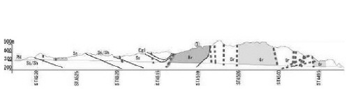
The actual tunnel in the new second Tomei-Meishin expressway is 3900 m long. Photo 1 shows a photograph of cutting face of actual tunnel. The standard cross-section of the actual tunnel in the new second Tomei-Meishin expressway is super large (200 m2) and wide (18 m) compared with ordinary tunnels. Fig. 7 shows the longitudinal geological cross-section.

6.1 Discontinuity measurement from unrolled trace map

The measurement from unrolled discontinuity trace map was performed (Hwang, 2003; Hwang et al., 2004). Fig. 8 shows the unrolled trace map of the TBM pilot tunnel of the actual tunnel. Fig. 9 shows the Schmidt net of discontinuities detected from unrolled trace map of the TBM pilot tunnel.

6.2 Key block prediction

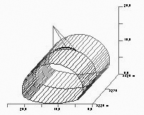
The prediction of key blocks using the proposed key block analysis method in actual tunnel was performed. The key blocks were predicted and prevented before the main tunnel excavation. In this section, to demonstrate the validity and applicability of the proposed system, the analytical results are compared and examined with results by common key block analysis method (the Japan Highway Public Corporation (JH) method (Hwang, 2003)). The key block analysis by the method stated earlier was based on the assumption of infinite persistent discontinuities, and considering the effects of discontinuity persistence was not possible using it. However, the key block analysis of this study considered finite persistence of discontinuities. The discontinuity information was acquired from the investigation of the advancing drift with TBM. The actual tunnel was modeled as shown in Fig. 10.

In this proposed method, the radii of discontinuity disks were determined to be 20 m and 45 m. The radii of discontinuity disks were determined by a trial and error method and the concept of representative elemental volume. The effects of scale on rock properties, occurring because of rock inhomogeneity and discontinuity, cause results on small-scale rock to be highly variable; this variability is increased by the presence of discontinuities. Indeed, one would not expect to obtain reproducible results for some of the properties unless the tests or analysis were on a scale such that the volume contained sufficiently representative discontinuities.

Table 1 shows the number of key blocks in STA. 527+50.0∼528+0.0. The distance between each STA. is 100 m. Two key blocks were predicted in STA. 527+50.0∼528+0.0. The number of key blocks in proposed method was exactly the same as that in the JH Method as shown in Table 1. The key block No.1 of this proposed method is compared with that of the JH method as shown in Fig. 11. Viewpoints in each key block are slightly different. However, the upper case key block No. 1 of this study shows a good match with that of the JH method. The comparisons and examinations with the analytical results have confirmed the validity and applicability of this proposed method in actual tunnels.

7. Conclusions

In this study, a new key block analysis method for observational design and construction method in tunnels is proposed, and then applied to the actual large tunnel with a super-large cross-section. Three-dimensional rock block identification with consideration of the persistence of discontinuities is performed by using discontinuity disk model. The new analysis method for observational design and construction method in tunnels can handle concave and convex shaped blocks. The developed key block analysis method considering discontinuity persistence for observational design and construction method consists of the following major steps: Discontinuity measurement from unrolled trace map, 3D discontinuous rock mass modeling, Identification of 2D loop, Identification of 3D loop, Finalization of block shape and volume, Removability and stability analysis of rock blocks.

To demonstrate the applicability of this key block analysis method for observational design and construction method in tunnels, the analysis results are examined and compared with those of the conventional method. The key block analysis by the proposed method in this study shows a good match with that by the conventional method. The comparisons and examinations with the analytical results have confirmed the validity and applicability of this developed analysis method in actual tunnels.